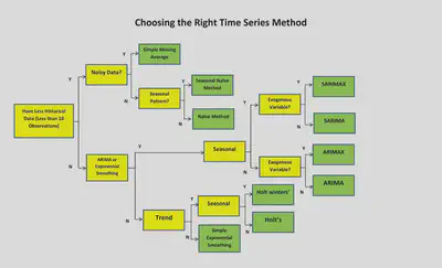
Time series analysis is a branch of statistics that deals with the analysis and interpretation of data that are collected over time. Time series data includes observations that are taken at regular intervals over time, such as stock prices, weather data, or economic indicators.
Time series analysis involves a range of techniques for describing and modeling time series data, such as time series decomposition, autocorrelation, and forecasting. These techniques can be used to explore the relationships between different time periods and to identify patterns and trends in the data.
Statistical models are also used in time series analysis to test hypotheses and make predictions about future observations. For example, autoregressive integrated moving average (ARIMA) models are commonly used to model and forecast time series data.
Time series analysis is widely used in various fields such as finance, economics, and engineering. It is also commonly used in machine learning and artificial intelligence applications, such as anomaly detection and prediction modeling.
Understanding and analyzing time series data is important for making informed decisions in many fields. Time series analysis provides a powerful set of tools for modeling, predicting, and interpreting time series data and is an essential tool for researchers, analysts, and decision-makers.
Python
import pandas as pd
import numpy as np
import matplotlib.pyplot as plt

# Load the data
df = pd.read_csv('time_series_data.csv', parse_dates=['Date'], index_col='Date')

# Check the data
print(df.head())

# Plot the time series data
plt.plot(df.index, df['Value'])
plt.xlabel('Date')
plt.ylabel('Value')
plt.title('Time Series Data')

# Resample the data to a monthly frequency
monthly_data = df.resample('M').mean()

# Plot the monthly data
plt.plot(monthly_data.index, monthly_data['Value'])
plt.xlabel('Date')
plt.ylabel('Value')
plt.title('Monthly Time Series Data')

# Decompose the time series data into trend, seasonality, and residuals
from statsmodels.tsa.seasonal import seasonal_decompose

decomposition = seasonal_decompose(df['Value'], model='additive')
trend = decomposition.trend
seasonal = decomposition.seasonal
residual = decomposition.resid

# Plot the decomposed time series data
plt.subplot(411)
plt.plot(df['Value'], label='Original')
plt.legend(loc='best')
plt.subplot(412)
plt.plot(trend, label='Trend')
plt.legend(loc='best')
plt.subplot(413)
plt.plot(seasonal,label='Seasonality')
plt.legend(loc='best')
plt.subplot(414)
plt.plot(residual, label='Residuals')
plt.legend(loc='best')
plt.tight_layout()

# Test for stationarity using the Augmented Dickey-Fuller test
from statsmodels.tsa.stattools import adfuller

result = adfuller(df['Value'])
print('ADF Statistic:', result[0])
print('p-value:', result[1])
print('Critical Values:', result[4])

# Perform first-order differencing to make the time series stationary
diff = df['Value'].diff().dropna()

# Plot the differenced time series data
plt.plot(diff)
plt.xlabel('Date')
plt.ylabel('Value')
plt.title('Differenced Time Series Data')

# Fit an ARIMA model to the time series data
from statsmodels.tsa.arima.model import ARIMA

model = ARIMA(df['Value'], order=(1, 1, 1))
results = model.fit()

# Print the model summary
print(results.summary())

# Forecast future values of the time series data
forecast = results.forecast(steps=12)

# Plot the forecasted values
plt.plot(forecast.index, forecast.values)
plt.xlabel('Date')
plt.ylabel('Value')
plt.title('Forecasted Time Series Data')
R
library(tidyverse)
library(lubridate)
library(forecast)
library(fpp2)

# Load the data
df <- read_csv("time_series_data.csv", col_types = cols(Date = col_datetime(format = "%Y-%m-%d"))) %>%
  mutate(Date = ymd(Date)) %>%
  as_tsibble(index = Date)

# Check the data
head(df)

# Plot the time series data
autoplot(df, y = Value) +
  labs(x = "Date", y = "Value", title = "Time Series Data")

# Resample the data to a monthly frequency
monthly_data <- df %>%
  index_by(Date) %>%
  summarise(Value = mean(Value)) %>%
  as_tsibble(index = Date)

# Plot the monthly data
autoplot(monthly_data, y = Value) +
  labs(x = "Date", y = "Value", title = "Monthly Time Series Data")

# Decompose the time series data into trend, seasonality, and residuals
decomposition <- stl(df$Value, s.window = "periodic")

# Plot the decomposed time series data
autoplot(decomposition)

# Test for stationarity using the Augmented Dickey-Fuller test
result <- adf.test(df$Value)
print(paste("ADF Statistic:", result$statistic))
print(paste("p-value:", result$p.value))
print(paste("Critical Values:", result$critical))

# Perform first-order differencing to make the time series stationary
diff <- diff(df$Value)

# Plot the differenced time series data
autoplot(ts(diff, start = start(df))) +
  labs(x = "Date", y = "Value", title = "Differenced Time Series Data")

# Fit an ARIMA model to the time series data
model <- Arima(df$Value, order = c(1, 1, 1))
results <- summary(model)

# Print the model summary
print(results)

# Forecast future values of the time series data
forecast <- forecast(model, h = 12)

# Plot the forecasted values
autoplot(forecast) +
  labs(x = "Date", y = "Value", title = "Forecasted Time Series Data")

Sophisticated approaches and models are necessary to tackle the intricacy of time series analysis. These can encompass nonlinear models, such as nonlinear autoregressive models, state-space models, and machine learning algorithms, including support vector regression and recurrent neural networks. Additionally, specialized methods such as wavelet analysis or Fourier transforms may also be applicable. The selection of an appropriate methodology should be guided by the data’s characteristics and the objectives of the analysis.
Time series analysis can be a challenging task due to the complexity of the data involved. To conduct a proper analysis, one needs to employ sophisticated models and techniques. For instance, nonlinear models like Autoregressive Neural Network and Nonlinear Autoregressive with eXogenous inputs can be used to model nonlinear time series data. State-space models are effective in capturing system dynamics over time while also considering external variables. Additionally, machine learning techniques like recurrent neural networks and support vector regression can be used to analyze time series data. To analyze the frequency content of time series data, specialized techniques such as wavelet analysis and Fourier transformations are useful. It’s crucial to choose the appropriate approach depending on the data characteristics and research objectives. The use of inappropriate methods may result in erroneous findings. On the other hand, using the right techniques can unlock the full potential of time series analysis and provide valuable insights into the behavior of dynamic systems.